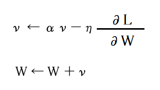
モーメンタムの数式

SGDの欠点を改善するために代わる手法としてモーメンタムがあります。
モーメンタムは、ボールが傾斜を転がるように動くイメージと言われています。数式にすると、以下のようになります。”ν”は速度を表しているそうです。
(数式の詳細な説明は「0からDeepLearning」を参照してください)
モーメンタムのサンプルプログラム
モーメンタムは、以下のような形で実現します。
数式はわからないですが、プログラムにするとよくわかりますね。
これで、ボールが、お椀の底を転がるような動きを再現できるというから不思議ですね。
class Momentum:
    def __init__(self, lr=0.01, momentum=0.9):
        self.lr = lr
        self.momentum = momentum
        self.v = None

    def update(self, params, grads):
        if self.v is None:
            self.v = {}
            for key, val in params.items():
                self.v[key] = np.zeros_like(val)

        for key in params.keys():
            self.v[key] = self.momentum*self.v[key] - self.lr*grads[key]
            params[key] += self.v[key]
モーメンタムのグラフ
最後にグラフがどのように表示されるのかをご紹介します。
このグラフは、以下のプログラムを実行した結果です。
確率的勾配降下法(SGD)と比べると、ジグザグ感がなくなっていますね。SGDより速く(0,0)の座標へ近づいているのがわかります。
import sys, os
sys.path.append(os.pardir)
import matplotlib.pyplot as plt
from collections import OrderedDict
from common.optimizer import *
def f(x, y):
    return x ** 2 / 20.0 + y ** 2
def df(x, y):
    return x / 10.0, 2.0 * y
init_pos = (-7.0, 2.0)
params = {}
params['x'], params['y'] = init_pos[0], init_pos[1]
grads = {}
grads['x'], grads['y'] = 0, 0
optimizers = OrderedDict()
optimizers["Momentum"] = Momentum(lr=0.1)
idx = 1
for key in optimizers:
    optimizer = optimizers[key]
    x_history = []
    y_history = []
    params['x'], params['y'] = init_pos[0], init_pos[1]
    for i in range(10000):
        x_history.append(params['x'])
        y_history.append(params['y'])
        grads['x'], grads['y'] = df(params['x'], params['y'])
        optimizer.update(params, grads)
    x = np.arange(-10, 10, 0.01)
    y = np.arange(-5, 5, 0.01)
    X, Y = np.meshgrid(x, y)
    Z = f(X, Y)
    # for simple contour line
    mask = Z > 7
    Z[mask] = 0
    # plot
    plt.subplot(1, 1, idx)
    idx += 1
    plt.plot(x_history, y_history, 'o-', color="red")
    plt.contour(X, Y, Z)
    plt.ylim(-10, 10)
    plt.xlim(-10, 10)
    plt.plot(0, 0, '+')
    # colorbar()
    # spring()
    plt.title(key)
    plt.xlabel("x")
    plt.ylabel("y")
plt.show()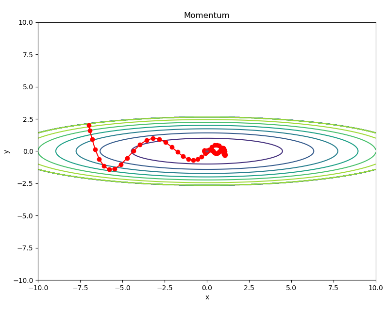
引用元
オライリーJapan 斎藤康毅 著 「セロから作るDeep Learning」